
Four ways to run a city's lighting, put side by side.
Fulda runs adaptively across the whole installation, split into sixteen projects. Between April and July 2025 we measured what it actually consumed — and worked out what the same luminaires would have consumed on the three strategies a city is usually offered instead.
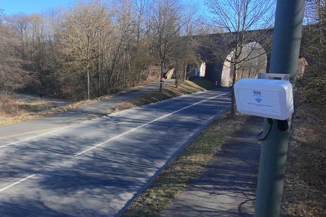
Street under adaptive control — installed site, Germany
The same city, on four different strategies.
Most tenders choose between these four. Rarely does anyone get to see them on the same installation, over the same months, with the same weather and the same traffic.
What is measured and what is computed.
The adaptive figure — 20.0 MWh — is metered: the nodes report their own energy, hour by hour, and it is added up. The other three are what the same luminaires would have drawn on those profiles over the same nights, computed from their power and the hours involved. We say which is which, because the difference matters when someone checks.
How we measure →Each percentage compares the same 20.0 MWh with a different starting point. They are not added together, and none of them is a saving on top of another.
The honest comparison for a city that has already relamped: 20.0 against 47.0 MWh. This is what adaptive control adds on top of the LED project.
The alternative most often written into a tender — dim everything to 40 % between 23:00 and 05:00 — brings 47.0 MWh down to 31.8, about a third. Adaptive operation then takes 37 % off what that profile leaves: 31.8 down to 20.0. The two effects multiply rather than add, and together they are the −58 % above.
The whole journey, LED retrofit included: 20.0 against 95.0 MWh. It is the biggest number and the least informative one — most of the first half was the lamp change, which any supplier would have done.
A city is not one average.
The installation is divided into sixteen adaptive projects, each covering streets of one kind. They do not all save the same, and that is the point: the saving follows the traffic a street actually carries.
From 31 % to 65 % against LED
Quiet streets with long empty hours save most; streets that stay busy save least. Against the previous HPS lamps the same projects range from 64 % to 86 %.
Three quarters of it above 50 %
More than 75 % of the installed load sits in projects saving over half against full-power LED — so the good result is not carried by a few small streets.
13 % of the load, −52 %
The project with the biggest share of the city's power saves 52 % against LED and 73 % against HPS — a solid result exactly where it counts most.
We left a fault in, so the number would be real.
One of the sixteen projects saved only 31 % against LED, against a typical 55–60 %. In that zone the dynamic profile had never been activated: the luminaires were running at a fixed level all night, as if nothing had been installed.
We found it during the window
The fix is a configuration change, a few minutes of work. Applying it would have improved the average in the middle of the evaluation period.
We postponed it on purpose
The three months were meant to measure what the system does, not what it does after we tidy it up. The intervention waited until the window closed.
It is in the figures you are reading
That project is 4 % of the installed load, and its weak result is inside the −58 % above. A measurement you can only reproduce on a good day is not a measurement.
Sensors on the street, decisions at the roadside.
Radar sensors count vehicles in both directions on the instrumented stretches; luminance is read on the road surface; a weather station reports rain, fog and snow. The lighting class is recalculated from those inputs, within what EN 13201 and UNI 11248 allow, and applied to the group over the mesh.
On the sampled stretch the design class is M2 — a main road — and the measured light level follows the traffic curve down through the night and back up before the morning peak, without ever dropping below what the standard permits for the conditions.
Adaptive lighting →The platform is operated by us and hosted in Germany. The city's data and its backups belong to the city, exported in standard formats whenever it asks — which is what data sovereignty means in a German tender, and it does not require the city to run a platform itself.
iLCS Cloud →Measured by us on the installation and written up in a technical report, available on request. Unlike our three Italian and Vietnamese cases, this one has not been through peer review — so we label it for what it is.
The published cases →A fixed night profile leaves 37 % on the table.
That is what this city would have paid for keeping it simple — every year, for the life of the installation. Send the road categories and the traffic you have, and we will tell you what the same comparison looks like on your network.